How to hide Grand Total row in Google Sheets Pivot Charts

This was driving me insane for the longest time. Its really easy to hide the grand totals in Excel but how to do it in Google Sheets?

As I was trying to come up with creative solutions using custom formulas, it dawned on me to try something really stupid simple just to see what happens.

There are two ways:

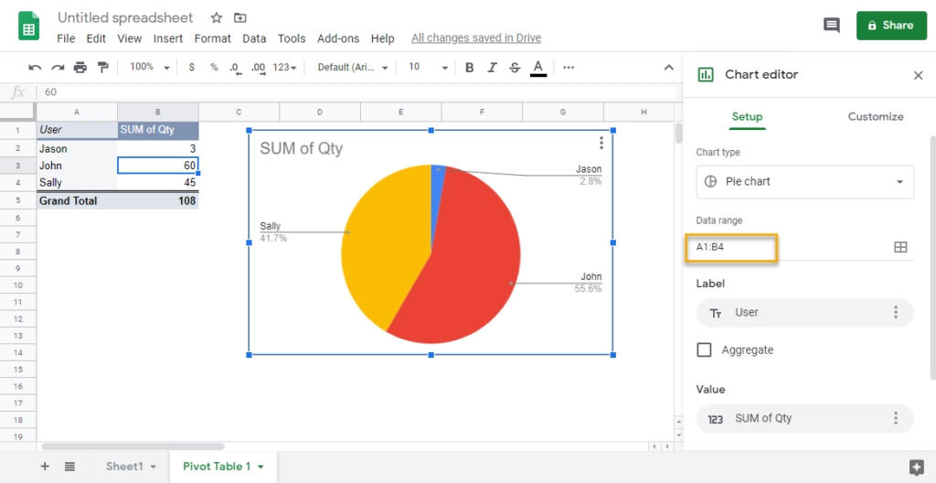
1. Update your Chart -> Setup -> Data range to only include the header rows and data.
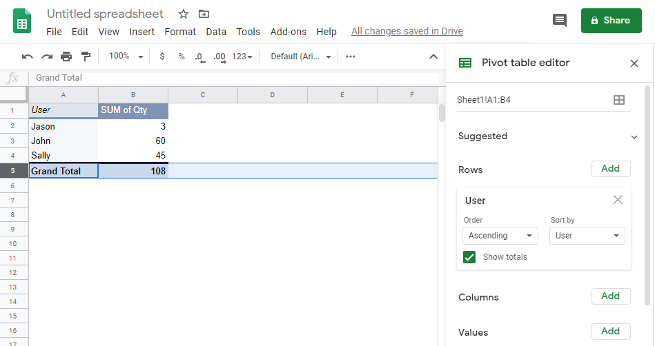
   1. For example my Pivot Table has the Grand Total in row 5
   2. In your Chart -> Setup -> Data range, update to A1:B4 to exclude row 5.
      

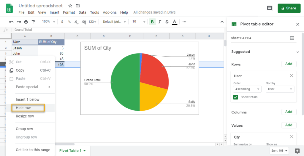
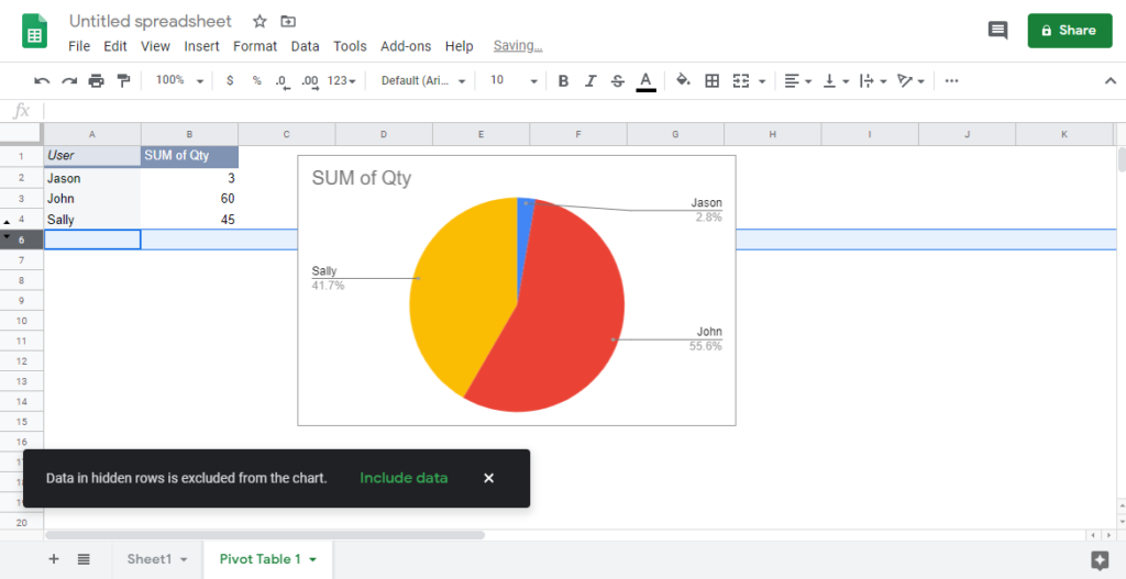
1. If you want to remove the Grand Total from both the Pivot table AND the Chart, simply Right click on the Grand Total row and choose Hide Row